Modeling the Human Sinoatrial Node

Introduction
Model Foundation
Prerequisites for Implementing the Human SAN Model
Python Code Generation from CellML File
Understanding the Structure of the Generated Python Code
Code Modifications
Conclusions
Outlook
References

1. Introduction

The heart’s rhythm, that steadfast beat echoing life’s very essence, begins in a specialized region known as the sinoatrial node (SAN). Understanding the SAN isn’t just a matter of anatomy; it’s about unraveling the electrical dance that initiates each heartbeat.

In 2017, a groundbreaking study by Alan Fabbri and colleagues [1] brought us closer to this understanding by constructing a comprehensive mathematical model of the human SAN pacemaker cell. Published in The Journal of Physiology, this work doesn’t merely echo the rhythm of life; it deciphers its code.

Basing their model on electrophysiological data from isolated human SAN pacemaker cells and building on the Severi-DiFrancesco model of rabbit SAN cells [2], Fabbri et al. crafted a mathematical portrait that closely resembles the action potentials and calcium transient found in real human cells.

But why does this matter? It's more than a scientific curiosity. The model provides insights into the "funny current" (I_f) that modulates the heart's pacing rate. It explains how certain mutations affect heart rate, a finding that resonates with clinical observations. And perhaps most excitingly, it offers a valuable tool for designing new experiments and developing drugs that can tune the heart's rhythm.

Today, I invite you to delve into the heart of this paper with me. Let’s explore the intricacies of the human SAN pacemaker cell, understand its rhythm, and appreciate the beauty of mathematical modeling in the realm of biology.

You can download the complete code of the SAN model from this article from our GitHub repository.

2. Model Foundation

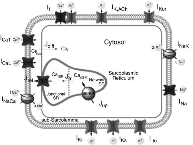
The starting point of the work by Fabbri et al. [1] was the rabbit SAN cell model from Severi et al. [2], developed as a Hodgkin-Huxley-type model. This model utilizes differential equations to describe how ionic current flow through the cell membrane gives rise to the electrical activity in the cell, providing a foundational approach to understanding membrane potential dynamics. The Fabbri et al. model [1] integrated enhancements derived from electrophysiological data of human cells, along with automatic optimization for unknown parameters. Influenced by various human cell data, it was constrained by AP parameters, voltage clamp data, effects of I_f blockers, and Ca²⁺ transient data. Figure 1 shows a schematic diagram of the human SAN AP model, emphasizing the compartmentalization essential for calcium handling and detailing the ionic currents, pumps, and exchangers inherited from the parent model or developed independently.

Figure 1 The cell is segmented into three areas: the subsarcolemma, cytosol, and sarcoplasmic reticulum (SR), with the SR further split into junctional and network sections. The handling of Calcium ions Ca²⁺ is facilitated by two diffusion processes \( (J_{\text{diff}}\), from subsarcolemmal to cytosol and \( J_{\text{tr}}\) from network SR to junctional SR, the uptake of Ca²⁺ into the network SR by the SERCA pump (\(J_{\text{up}}\)), and the release of Ca²⁺ from the junctional SR into the subsarcolemmal space through RyRs. There are 11 various ionic channels, pumps, and exchangers through which Sodium, Calcium, and Potassium ions move across the sarcolemmal membrane. Reproduced from Fabbri et al. [1, p.2367]

2.1. Membrane Potential Dynamics in the Human SAN Model

The essence of modeling the electrical activity of the SAN cell is captured in the representation of the membrane potential, \( V \), which describes the voltage difference across the cell membrane. This potential is the driving force behind the flow of ions through various channels and pumps, and it orchestrates the complex rhythm of the heart's natural pacemaker.

In the Hodgkin-Huxley-type models, including the one utilized by Fabbri et al. [1], the membrane potential is described by a differential equation that considers the cumulative effects of multiple ionic currents (Table 1). These currents, each mediated by specific channels or exchangers, contribute to the overall charge movement across the membrane.

The membrane potential equation for the human SAN cell model is given by:

\[ \frac{dV}{dt} = -\frac{1}{C} \cdot \left( I_{\text{f}} + I_{\text{CaL}} + I_{\text{CaT}} + I_{\text{Kr}} + I_{\text{Ks}} + I_{\text{K,ACh}} + I_{\text{to}} + I_{\text{Na}} + I_{\text{NaK}} + I_{\text{NaCa}} + I_{\text{Kur}} \right) \]

Here, \( \frac{dV}{dt} \) is the rate of change of the membrane potential with respect to time, \( C \) is the membrane capacitance, and the terms inside the parentheses represent the various ionic currents that play a vital role in the depolarization and repolarization phases of the action potential.

This equation elegantly encapsulates the interactions and dynamics of the SAN cell membrane, highlighting the role of each ion channel in generating the characteristic rhythmic electrical activity of the SAN.

Current	Description
\(I_{\text{f}}\)	Funny current
\(I_{\text{CaL}}\)	L-type calcium current
\(I_{\text{CaT}}\)	T-type calcium current
\(I_{\text{Kr}}\)	Rapid delayed rectifier potassium current
\(I_{\text{Ks}}\)	Slow delayed rectifier potassium current
\(I_{\text{K,ACh}}\)	Potassium current modulated by acetylcholine
\(I_{\text{to}}\)	Transient outward potassium current
\(I_{\text{Na}}\)	Sodium current
\(I_{\text{NaK}}\)	Sodium-potassium pump current
\(I_{\text{NaCa}}\)	Sodium-calcium exchanger current
\(I_{\text{Kur}}\)	Ultra-rapid delayed rectifier potassium current

Table 1 Ionic Currents in the Human SAN Model.

2.2. Understanding Ion Channel Dynamics: A Look at the Hodgkin-Huxley Model

While the modeling of the human sinoatrial node cell is multifaceted, the core concept of how an ion channel is modeled can be elucidated through the example of the sodium (Na⁺) channel in infamous the Hodgkin-Huxley model. In this well-known model, the Na⁺ channel's behavior is governed by specific gating variables, and the flow of Na⁺ ions across the membrane is given by the equation:

The Hodgkin-Huxley model elegantly describes the membrane potential of a neuron by considering the flow of sodium (Na⁺), potassium (K⁺), and leak currents. The total current flowing through the membrane is given by the equation:

\[ \frac{dV}{dt} = \frac{1}{C_m} \cdot (I_{\text{ext}} - (I_{\text{Na}} + I_{\text{K}} + I_{\text{L}})) \]

where

\( V \) is the membrane potential,
\( C_m \) is the membrane capacitance,
\( I_{\text{ext}} \) is an external current,
\( I_{\text{Na}} \) is the sodium current,
\( I_{\text{K}} \) is the potassium current,
\( I_{\text{L}} \) is the leak current.

While the modeling of the human sinoatrial node cell is multifaceted, the core concept of how an ion channel is modeled can be elucidated through the example of the sodium (Na⁺) channel in the Hodgkin-Huxley model. In this well-known model, the Na⁺ channel's behavior is governed by specific gating variables, and the flow of Na⁺ ions across the membrane is given by the equation:

\[ I_{\text{Na}} = g_{\text{Na}} \cdot m^3 \cdot h \cdot (V - E_{\text{Na}}) \]

where

\( I_{\text{Na}} \) is the sodium current,
\( g_{\text{Na}} \) is the maximum sodium conductance,
\( m \) is the activation gate variable,
\( h \) is the inactivation gate variable,
\( V \) is the membrane potential,
\( E_{\text{Na}} \) is the sodium Nernst potential.

The time evolution of the gating variables 'm' and 'h' is described by:

\[ \frac{dm}{dt} = \alpha_m(V) \cdot (1-m) - \beta_m(V) \cdot m \]

\[ \frac{dh}{dt} = \alpha_h(V) \cdot (1-h) - \beta_h(V) \cdot h \]

The table below (Table 2) summarizes these parameters with their common values.

Parameter	Description	Common Values
\( C_m \)	Membrane capacitance	1 μF/cm²
\( g_{\text{Na}} \)	Maximum sodium conductance	120 mS/cm²
\( E_{\text{Na}} \)	Sodium Nernst potential	+115 mV
\( \alpha_m \)	Rate constant for m activation	Varies with \( V \)
\( \beta_m \)	Rate constant for m inactivation	Varies with \( V \)
\( \alpha_h \)	Rate constant for h activation	Varies with \( V \)
\( \beta_h \)	Rate constant for h inactivation	Varies with \( V \)

Table 2 Parameters used in the Hodgkin-Huxley model, including descriptions and common values for the sodium channel and membrane capacitance.

By exploring the intricacies of the Na⁺ channel within the Hodgkin-Huxley framework, we can glean essential insights into how ion channels are implemented, providing a foundational understanding that extends to more complex models like those of the human sinoatrial node cell.

2.3. Cell Capacitance and Dimensions

Cell dimensions and membrane capacitance were assumed in line with experimental data, adopting dimensions of intracellular compartments from the parent model [2].

2.4. Membrane Currents

Fabbri et al. [1] specified sarcolemmal currents flowing through ionic channels, pumps, and exchangers shown in Figure 1, except for \(I_{K,ACh}\). Adjustments were made for various currents such as the funny current (\(I_f\)), rapid delayed rectifier K⁺ current (\(I_{Kr}\)), slow delayed rectifier K⁺ current (\(I_{Ks}\)), ultrarapid delayed rectifier K⁺ current (\(I_{Kur}\)), and others. These modifications included changes in conductance, implementation of kinetic schemes, and adjustments based on experimental findings or automatic optimization.

2.5. Calcium Handling

The mathematical formulation of Ca²⁺ handling was maintained from the parent model [2], but parameters were updated through automatic optimization, including aspects such as SR Ca²⁺ uptake (\(J_{up}\)), SR Ca²⁺ release (\(J_{rel}\)), and Ca²⁺ diffusion and buffers.

2.6. Ion Concentrations

The model by Fabbri et al. included a detailed description of Ca²⁺ dynamics for four compartments and fixed intracellular Na⁺ concentration, following the whole cell configuration used in certain experiments.

Overall, the model by Fabbri et al. [1] integrates detailed revisions to accurately represent human SAN cells, reflecting experimental data, and making specific modifications to currents, capacitance, Ca²⁺ handling, and ion concentrations.

2.7. Autonomic Modulation of the Sinoatrial Node

The autonomic modulation of the SA node is a critical aspect of cardiac function, allowing the heart rate to be precisely regulated in response to various physiological demands. The autonomic nervous system (ANS) influences the SA node through both its sympathetic and parasympathetic branches. Sympathetic stimulation increases the heart rate by enhancing the pacemaker currents within the SA node, preparing the body for stress or physical activity. In contrast, parasympathetic stimulation, mediated mainly through acetylcholine, reduces the heart rate by inhibiting these currents, promoting a state of rest and recovery. The balance between these two branches ensures that the heart rate is finely tuned to meet the body's needs, whether it is responding to exercise, stress, or relaxation. The modulation of the SA node by the ANS is a complex interaction involving neurotransmitters, receptors, ionic channels, and cellular signaling pathways. It is a fundamental aspect of cardiovascular regulation, with implications for overall heart health and disease management.

The effects of 10 nM ACh on \(I_{f}\) activation (–7.5 mV shift in voltage dependence of activation), \(I_{CaL}\) (3.1% reduction of maximal conductance) and SR Ca\(^{2+}\) uptake (7% decrease of maximum activity) were all adopted from the parent model [2]. The administration of ACh also activates \(I_{K,ACh}\), which is zero in the default model. The \(I_{K,ACh}\) formulation was derived from the parent model. The maximal conductance \(g_{K,ACh}\) was set to 3.45 nS (reduced by 77.5%) to achieve an overall reduction of the spontaneous rate by 20.8% upon administration of 10 nM ACh, as observed by Bucchi et al. [3] in rabbit SAN cells. The targets of isoprenaline (Iso), an antagonist of the sympathetic neurotransmitter Noradrenaline, are \(I_{f}\), \(I_{CaL}\), \(I_{NaK}\), maximal Ca\(^{2+}\) uptake and \(I_{Ks}\). Changes in currents were adopted from the parent model, except for the modulation of \(I_{CaL}\), where the effect of Iso induced a slightly smaller decrease of the slope factor \(k_{dL}\) (–27% with respect to control conditions, instead of the –31% assumed by the parent model). The \(I_{CaL}\) current was modulated to fit the experimental data reported by Bucchi et al. [3] on rabbit SAN cells (26.3±5.4%; mean±SEM, n=7) for the same Iso concentration [1].

2.8. Action Potential Waveform

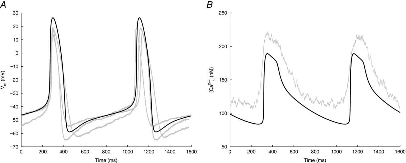
The simulated action potential (AP) waveform has been shown to be in good alignment with the available experimental data, as depicted in Figure 2. The majority of the quantitative factors that detail the morphology of the AP, including cycle length (CL), MDP (maximum diastolic potential), APD₉₀ (action potential duration at 90% repolarization), and DDR₁₀₀ (100% diastolic depolarization rate), fall within the mean ± SD (standard deviation) range of the experimentally observed values [4]. Specifically, the model's AP is defined by a CL of 814 ms, corresponding to a beating frequency of 74 beats per minute. Notably, the model displays a higher (dV/dt)_max and overshoot (OS), and a more prolonged APD₂₀, which are predicted characteristics outside the experimental mean ± SD range.

Figure 2 (A) The simulated action potential of a single human SAN (sinoatrial node) cell is shown as a black thick line, contrasted with the experimentally recorded action potentials from three individual isolated human SAN cells, represented by the grey traces. The experimental data were sourced from Verkerk et al. [4] and Verkerk and Wilders [5]. (B) A comparison between the simulated (black thick line) and experimentally recorded (grey line) Ca²⁺ transient is depicted. Experimental data for this was obtained from Verkerk et al. [6]. Reproduced from Fabbri et al. [1, p.2373]

3. Prerequisites for Implementing the Human SAN Model

Before we dive into the heart of the modeling, there are some essential tools and resources you'll need to have ready:

Python: The beating core of our code, Python is the programming language we'll use to bring this model to life. If you don't already have it installed, you can download it from the official Python website.
Python Packages: These libraries act as the supporting vessels for our code:
- numpy: For numerical computations.
- scipy: To leverage scientific and technical computing.
- matplotlib: To visualize the results and plot beautiful graphs.
OpenCOR Software: This tool allows us to export the CellML model as Python, bridging the gap between biological understanding and computational implementation. Download OpenCOR at this link.
CellML Model of Fabbri et al.: The specific blueprint we'll be exploring, this model is key to our journey. You can find it readily available at this location.

Note: You can install the Python packages using the following command:

$ pip install numpy scipy matplotlib

Once you've gathered these components, you'll be well-prepared to follow along as we explore the computational intricacies of the human sinoatrial node model.

4. Python Code Generation from CellML File

Generating Python code from a CellML file is a straightforward process, and OpenCOR makes it a breeze. With just one command, you can transform the Fabbri model into executable Python code. Here's how:

Open your command line or shell interface.
Navigate to the directory where OpenCOR and the CellML file are located.
Open your shell and execute the following command to generate a Python file from the specified CellML model:

$ ./OpenCOR -c CellMLTools::export HumanSAN_Fabbri_Fantini_Wilders_Severi_2017.cellml python.xml

If you'd like to dive deeper into the code generation process and explore additional options, more detailed information is available on the OpenCOR website.

With the code successfully generated, you're ready to move on to the next steps, including model simulation and analysis. Let's get coding!

5. Understanding the Structure of the Generated Python Code

This section offers an in-depth examination of the Python code generated to simulate the sinoatrial node. The code is structured into various functions, each tailored to handle distinct aspects of the SAN model. Below, each function is presented with a description of its purpose.

5.1. Size Definitions and Imports

This part of the code defines the sizes of various arrays that will be used throughout the code. It also imports all the functions from the math and NumPy modules.

from math import *
from numpy import *
# Variable array sizes
sizeAlgebraic = 101
sizeStates = 33
sizeConstants = 116

5.2. Create Legends and Labels

The createLegends function initializes and sets legends or descriptions for states, algebraic variables, variable of integration (voi) or time, and constants. This can be useful for annotating plots or for providing context to the values within the code.

def createLegends():
    legend_states = [""] * sizeStates
    legend_rates = [""] * sizeStates
    legend_algebraic = [""] * sizeAlgebraic
    legend_voi = ""
    legend_constants = [""] * sizeConstants
    legend_voi = "time in component environment (second)"
    legend_constants[0] = "R in component Membrane (joule_per_kilomole_kelvin)"
    legend_constants[1] = "T in component Membrane (kelvin)"
    legend_constants[2] = "F in component Membrane (coulomb_per_mole)"
    legend_constants[3] = "C in component Membrane (microF)"
    legend_constants[91] = "RTONF in component Membrane (millivolt)"
    legend_algebraic[59] = "i_f in component i_f (nanoA)"
    ...
    return legend_states, legend_algebraic, legend_voi, legend_constants

5.3. Initialize Constants and States

The initConsts function initializes the constants and states arrays. The constants are values that do not change during the simulation, whereas the states represent the initial state of the system and can be altered as the system evolves.

def initConsts():
    constants = [0.0] * sizeConstants; states = [0.0] * sizeStates;
    constants[0] = 8314.472
    constants[1] = 310
    constants[2] = 96485.3415
    constants[3] = 5.7e-5
    constants[4] = 0
    states[0] = -47.787168
    constants[5] = 0.5
    constants[6] = 0.5
    constants[7] = -35
    ...
    return states, constants

5.4. Compute Rates

The computeRates function computes the rate of change of the states based on the current values of states, constants, and variable of integration (voi). This function is essential for the numerical integration step where the system evolves over time.

def computeRates(voi, states, constants):
    rates = [0.0] * sizeStates; algebraic = [0.0] * sizeAlgebraic
    algebraic[6] = constants[69]*constants[78]*(1.00000-(states[22]+states[18]))-constants[75]*states[18]
    rates[18] = algebraic[6]
    algebraic[1] = constants[47]/(constants[47]+states[1])
    algebraic[7] = (0.00100000*algebraic[1])/constants[46]
    rates[8] = (algebraic[1]-states[8])/algebraic[7]
    algebraic[2] = constants[51]-(constants[51]-constants[52])/(1.00000+power(constants[53]/states[15], constants[54]))
    algebraic[8] = constants[55]/algebraic[2]
    algebraic[17] = constants[56]*algebraic[2]
    rates[11] = (constants[57]*states[14]-algebraic[17]*states[1]*states[11])-(algebraic[8]*(power(states[1], 2.00000))*states[11]-constants[58]*states[12])
    rates[12] = (algebraic[8]*(power(states[1], 2.00000))*states[11]-constants[58]*states[12])-(algebraic[17]*states[1]*states[12]-constants[57]*states[13])
    ...
    return rates

5.5. Compute Algebraic Variables

The computeAlgebraic function computes algebraic variables, which are derived from the state variables but are not part of the differential equations themselves. These can represent various quantities of interest in the model.

def computeAlgebraic(constants, states, voi):
    algebraic = array([[0.0] * len(voi)] * sizeAlgebraic)
    states = array(states)
    voi = array(voi)
    algebraic[6] = constants[69]*constants[78]*(1.00000-(states[22]+states[18]))-constants[75]*states[18]
    algebraic[1] = constants[47]/(constants[47]+states[1])
    algebraic[7] = (0.00100000*algebraic[1])/constants[46]
    algebraic[2] = constants[51]-(constants[51]-constants[52])/(1.00000+power(constants[53]/states[15], constants[54]))
    algebraic[8] = constants[55]/algebraic[2]
    algebraic[17] = constants[56]*algebraic[2]
    algebraic[5] = custom_piecewise([greater(voi , constants[5]) & less(voi , constants[5]+constants[6]), constants[7] , True, constants[8]])
    ...
    return algebraic

5.6. Piecewise Function

The custom_piecewise function computes the result of a piecewise-defined function. It takes as input a list of conditions and values and returns the value corresponding to the first true condition.

def custom_piecewise(cases):
    """Compute result of a piecewise function"""
    return select(cases[0::2],cases[1::2])

5.7. Solve the Model

The solve_model function sets up and solves the differential equations using SciPy’s ODE solver. It initializes the constants and states, sets up the solver, and then integrates the system over a specified time span, returning the variable of integration, states, and algebraic variables.

def solve_model():
    """Solve model with ODE solver"""
    from scipy.integrate import ode
    # Initialise constants and state variables
    (init_states, constants) = initConsts()

    # Set timespan to solve over
    voi = linspace(0, 10, 500)

    # Construct ODE object to solve
    r = ode(computeRates)
    r.set_integrator('vode', method='bdf', atol=1e-06, rtol=1e-06, max_step=1)
    r.set_initial_value(init_states, voi[0])
    r.set_f_params(constants)

    # Solve model
    states = array([[0.0] * len(voi)] * sizeStates)
    states[:,0] = init_states
    for (i,t) in enumerate(voi[1:]):
        if r.successful():
            r.integrate(t)
            states[:,i+1] = r.y
        else:
            break

    # Compute algebraic variables
    algebraic = computeAlgebraic(constants, states, voi)
    return voi, states, algebraic

5.8. Plot the Results

The plot_model function plots the state and algebraic variables against the variable of integration. It can be used to visualize the evolution of the system over time.

def plot_model(voi, states, algebraic):
    """Plot variables against variable of integration"""
    import pylab
    (legend_states, legend_algebraic, legend_voi, legend_constants) = createLegends()
    pylab.figure(1)
    pylab.plot(voi, vstack((states,algebraic)).T)
    pylab.xlabel(legend_voi)
    pylab.legend(legend_states + legend_algebraic, loc='best')
    pylab.show()

5.9. Main Execution

This part of the code is executed when the script is run directly. It calls the solve_model function to compute the results and then plots them using Matplotlib.

if __name__ == "__main__":
    (voi, states, algebraic) = solve_model()
    from matplotlib import pyplot as plt
    import numpy as np
    plt.plot(states)
    plt.xlim(0,20)
    plot_model(voi, states, algebraic)

In summary, this code defines a system of differential equations and provides functions to initialize the system, compute the derivatives, integrate the system over time, and plot the results. The code is organized into clear functions, each with a specific role in the modeling and simulation process.

6. Code Modifications

Unfortunately, the generated code does not work out of the box, requiring some critical adjustments. This situation often occurs when automatically produced code is utilized, and it highlights the necessity of human intervention in the coding process. In brief, the following actions will be undertaken to modify the existing code to make it functional and more user-friendly:

Refactoring for Readability: To enhance understanding and maintenance, the code will undergo refactoring. This process involves restructuring the existing code without changing its external behavior. It aims to improve the nonfunctional attributes of the software, making the code more readable.
Integration with SciPy's solve_ivp: The existing solver will be replaced with solve_ivp from the SciPy library. This modification will enhance the code's efficiency, leveraging a well-optimized solver. It necessitates adapting the function signatures and updating the way the model's differential equations are defined.
Plotting Code Modification: To generate a better-readable figure of the states, the existing plotting code will be modified. This may involve changes in labeling, scales, and visualization styles to convey the information more effectively.
Object Orientation: Shifting the code structure to an object-oriented paradigm to enhance the usability and manageability of the model.

These modifications will be vital to transform the raw generated code into a functional, efficient, and user-friendly script. The following sections will delve into each of these modifications, providing specific examples and guidance on implementing these changes. By following these steps, users will be able to leverage the provided code to suit their specific needs and preferences.

6.1. Definition of Sinoatrial Node Class

This section of the code defines the SinoAtrialNode class, allowing for the creation of a SAN object, which represents a central component of the heart's electrical system. This class structure enables encapsulation and modularity within the code.

In the SAN model, ACh and Nor represent the concentrations of acetylcholine and norepinephrine, respectively, two neurotransmitters that play crucial roles in the regulation of heart rate. Acetylcholine (ACh) is usually involved in slowing down the heart rate by reducing the pacemaker current, while norepinephrine (Nor) tends to increase the heart rate by enhancing the pacemaker current. These neurotransmitters interact with specific receptors in the cardiac cells, modulating the ionic currents and thus the overall behavior of the SAN. In the context of the model, the constants c[9] and c[10] are assigned to ACh and Nor respectively, allowing their concentrations to be manipulated and thus to simulate various physiological conditions, such as stress or relaxation, that would alter the concentrations of these neurotransmitters.

class SinoAtrialNode:
    def __init__(self, ACh=0, Nor=0):
        self.NUM_ALGEBRAIC = 101
        self.NUM_STATES = 33
        self.NUM_CONSTANTS = 116
        self.c = np.zeros(self.NUM_CONSTANTS)
        self.y = np.zeros(self.NUM_STATES)
        self.update(ACh, Nor)

6.2. Refactoring for Better Readability

The variables STATES, ALGEBRAIC, CONSTANTS are refactored to y, a, c, respectively, to improve readability and succinctness within the code. This change simplifies variable names without losing the underlying meaning.

self.c = np.zeros(self.NUM_CONSTANTS)
self.y = np.zeros(self.NUM_STATES)

6.3. Introduction of Update Function

An update function has been introduced that recalculates constants when ACh and Nor are adjusted. This function is called within the constructor, ensuring that the constants are properly initialized based on the given inputs.

def update(self, ACh, Nor):
    self.y[0] = -47.787168
    self.y[1] = 6.226104e-5
    self.y[2] = 5
    self.y[3] = 0.009508
    self.y[4] = 0.447724
    self.y[5] = 0.003058
    ...

6.4. Constructor for Initialization

The constructor method initializes all variables, including arrays for states and constants. This method sets up the initial state of the Sinoatrial Node object and ensures that it is ready for further operations.

def __init__(self, ACh=0, Nor=0):
    self.NUM_ALGEBRAIC = 101
    self.NUM_STATES = 33
    self.NUM_CONSTANTS = 116
    self.c = np.zeros(self.NUM_CONSTANTS)
    self.y = np.zeros(self.NUM_STATES)
    self.update(ACh, Nor)

6.5. Step Function for Calculating Rates

The step function calculates the rates for each step as the model advances in time. This function represents the dynamics of the system and updates the states based on the provided inputs and current state.

def step(self, t, y):
    a = np.zeros(self.NUM_ALGEBRAIC)
    dydt = np.zeros(self.NUM_STATES)
    self.y = y
    a[6] = self.c[69] * self.c[78] * (1.0 - (self.y[22] + self.y[18])) - self.c[75] * self.y[18]
    dydt[18] = a[6]
    a[1] = self.c[47] / (self.c[47] + self.y[1])
    a[7] = (0.001 * a[1]) / self.c[46]
    dydt[8] = (a[1] - self.y[8]) / a[7]
    ...
    return dydt

6.6. Conversion of Piecewise Terms to Use NumPy

The original code contained custom piecewise functions generated by the OpenOCR code generator. In this modification, those custom piecewise functions were replaced with NumPy's built-in np.piecewise function. This change leverages the efficiency and readability of NumPy's functions and ensures compatibility with other NumPy-based calculations within the code.

# Example usage of np.piecewise in the code
result = np.piecewise(x, [condition1, condition2], [value_if_condition1, value_if_condition2])

6.7. Executing the Simulation with `solve_ivp`

The simulation of the Sinoatrial Node model is executed using SciPy's solve_ivp function, a general-purpose solver for initial value problems with a flexible interface for defining complex systems of ordinary differential equations (ODEs).

import SinoAtrialNode
import numpy as np
from scipy.integrate import solve_ivp

tmax = 5  # simulation duration
san = SinoAtrialNode.SinoAtrialNode()  # generate the sinoatrial node object 
sol = solve_ivp(san.step, [0, tmax], list(san.y), method='BDF', rtol=1e-6,
                     t_eval=np.arange(0, tmax, 1e-4), vectorized=False)  # solve system

This call to solve_ivp integrates the model over the specified time interval, utilizing the BDF method and the provided initial conditions, tolerances, and evaluation points to generate the simulation results.

Here's a breakdown of the parameters used in the function:

san.step: This is the step function defined in the SinoAtrialNode class, responsible for calculating the rates at which the model advances in time.
[0, tmax]: Specifies the time span of integration, from 0 to tmax (5 in this example), indicating the start and end times of the simulation.
list(san.y): The initial conditions, defined as the initial state variables y from the Sinoatrial Node object.
method='BDF': Specifies the solver method to be used. The 'BDF' (Backward Differentiation Formula) method is an implicit multi-step method suitable for stiff problems.
rtol=1e-6: The relative tolerance parameter, determining the accuracy of the solution.
t_eval=np.arange(0, tmax, 1e-4): Defines the time points at which the solution is stored. It allows control over the discrete points in time for which the solver should return the system state.
vectorized=False: Indicates whether the function is implemented in a vectorized fashion. Setting this to False means that the function expects the input to be a single point in time.

6.8. Plotting the Results

The following code is used to visualize the simulation results. It includes the definition of the legend labels for the different states and plots all 33 states, each in a separate subplot.

import matplotlib.pyplot as plt

legend_states = [
    "V_ode in Membrane (mV)",
    "Ca_sub in Ca_dynamics (mM)",
    "Nai_ in Nai_concentration (mM)",
    ...
]

plt.figure(figsize=(20, 50))
for i in range(1, 33):
    plt.subplot(17,2,i)
    plt.plot(sol.t, sol.y[i-1])
    plt.ylabel(legend_states[i-1], fontsize=10)
    plt.xlabel("Time (s)")

plt.show()

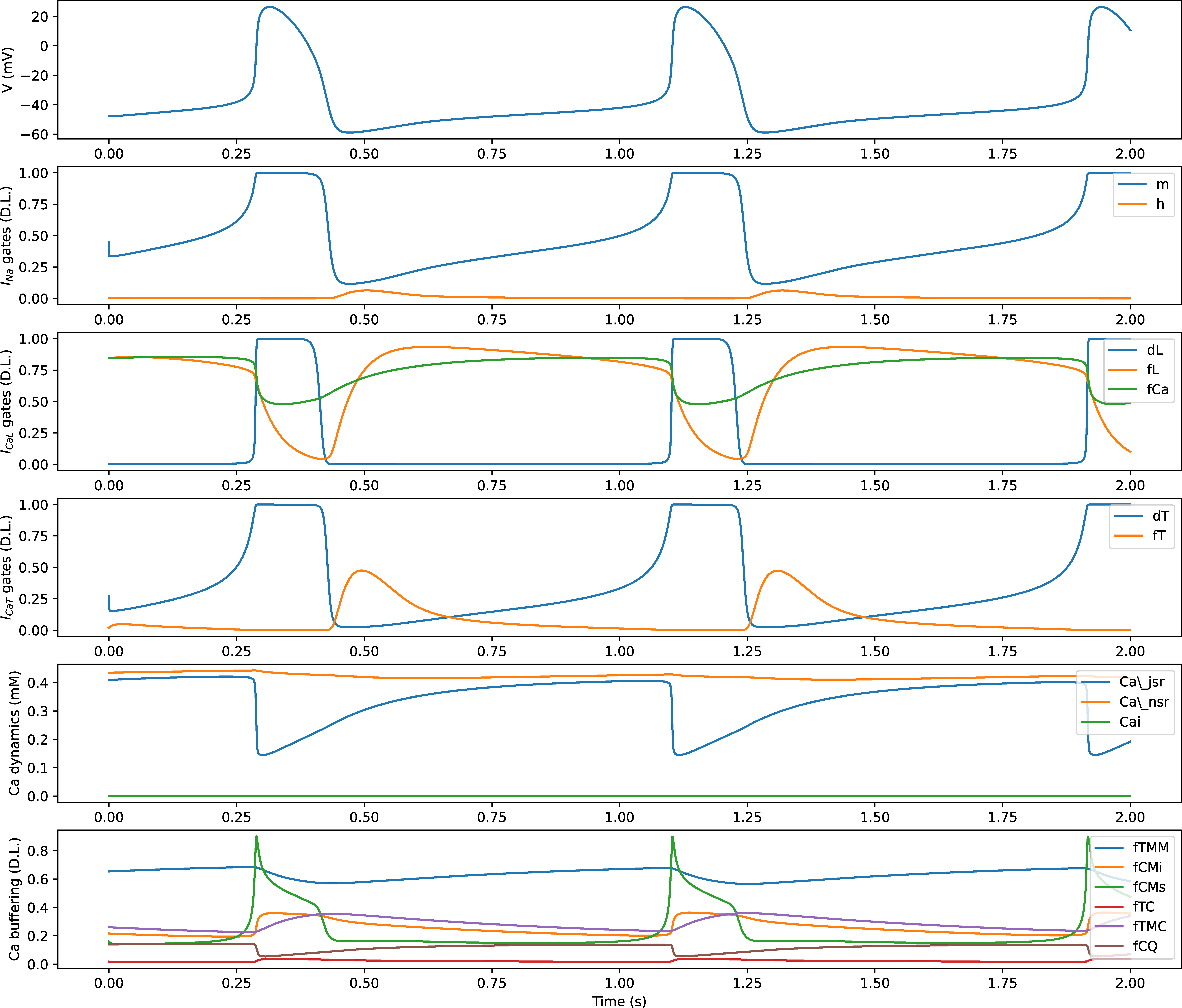
The code produces a figure with 9 subplots, representing selected essential states of the model, including membrane voltage \( V \), submembrane calcium concentration \( \text{Ca}_{\text{sub}} \), gating variables for sodium \( (m, h) \), L-type calcium \( (d_{L}, f_{L}, f_{\text{Ca}}) \), T-type calcium \( (d_{T}, f_{T}) \), and calcium dynamics in junctional and network sarcoplasmic reticulum \( (\text{Ca}_{\text{jsr}}, \text{Ca}_{\text{nsr}}) \) and intracellular calcium \( \text{Ca}_{i} \) (Figure 3).

The figure has been simplified to include only 9 subplots to focus on the most essential and representative states of the model (Figure 3). These selected states include key variables such as membrane voltage \( V \), submembrane calcium concentration \( \text{Ca}_{\text{sub}} \), and gating variables for different ionic currents that play a vital role in understanding the cell's electrophysiology. By concentrating on these states, the plot provides a clearer and more concise visualization, avoiding the complexity that would arise from including all 33 states.

Figure 3 This figure illustrates the time evolution of key states in the SAN cell model, including the membrane voltage \( V \), submembrane calcium concentration \( \text{Ca}_{\text{sub}} \), and gating variables for different ionic currents such as sodium \( (m, h) \), L-type calcium \( (d_{L}, f_{L}, f_{\text{Ca}}) \), T-type calcium \( (d_{T}, f_{T}) \), and calcium dynamics in junctional and network sarcoplasmic reticulum \( (\text{Ca}_{\text{jsr}}, \text{Ca}_{\text{nsr}}) \) and intracellular calcium \( \text{Ca}_{i} \). The selected states provide an insightful overview of the system's dynamics without the complexity of all 33 states. In the figure, the units and abbreviations used are as follows: \( mV \) stands for millivolts, representing the membrane voltage; \( mM \) denotes millimolar, a concentration unit used for calcium and other ions; and \( D.L. \) refers to dimensionless units, often utilized for gating variables that range from 0 to 1.

7. Conclusions

The complete code of the SAN model can be found in our GitHub repository. We welcome your insights and collaboration.

Here's a summary of the main lessons:

Understanding the Fundamental Principles of the SAN Model: We have laid out the core concepts and mechanisms behind the SAN model, diving into its intricacies and how it represents the beating of the heart.
Modeling Ion Channels in the Hodgkin-Huxley Type Model: By examining the Hodgkin-Huxley model, we've learned how ion channels are effectively portrayed in the cell membrane, shedding light on the cell's electrophysiology.
Exporting a CellML Model to Python Code: We have uncovered how a CellML model can be converted into Python, paving the way for efficient simulations and analysis.
Modifying the Code for Execution: Through hands-on examples, we've learned how to adjust and tweak the code to make it run smoothly.
Encapsulation through Object Orientation: By adopting object-oriented principles, we've streamlined the model into an encapsulated form, enhancing its modularity and reusability.
Solving the Model with Scipy's solve_ivp Solver: We've used Scipy's powerful solve_ivp solver to crunch the equations, gaining insights into the numerical techniques for solving differential equations.
Visualizing the Results: Finally, we've ventured into the art of data visualization, learning how to present the results of the model in a way that is both informative and visually appealing.

8. Outlook

Alright, folks, buckle up! Now that we've got our shiny Python implementation of the SAN model, things are about to get wild! 🚀 Next stop: Exploring the thrilling world of noradrenaline and acetylcholine. How do these sassy molecules shape the depolarization rate of the sinoatrial node? Hold onto your lab coats, because we're diving into that mystery in the next blog post. Get ready for a heart-pounding adventure that's bound to get your pulse racing! 🧪💓

Stay tuned, and keep those neurons firing! 🧠💥

References

Blog Archive

Archive of all previous blog posts

References

- Fabbri, Alan, et al. "Computational analysis of the human sinus node action potential: model development and effects of mutations." The Journal of physiology 595.7 (2017): 2365-2396.
- Severi, Stefano, et al. "An updated computational model of rabbit sinoatrial action potential to investigate the mechanisms of heart rate modulation." The Journal of physiology 590.18 (2012): 4483-4499.
- Bucchi, Annalisa, et al. "Modulation of rate by autonomic agonists in SAN cells involves changes in diastolic depolarization and the pacemaker current." Journal of molecular and cellular cardiology 43.1 (2007): 39-48.
- Verkerk, Arie O., et al. "Pacemaker current (I f) in the human sinoatrial node." European heart journal 28.20 (2007): 2472-2478.
- Verkerk, Arie O., and Ronald Wilders. "Relative importance of funny current in human versus rabbit sinoatrial node." Journal of Molecular and Cellular Cardiology 48.4 (2010): 799-801.
- Verkerk, Arie O., Marcel MGJ van Borren, and Ronald Wilders. "Calcium transient and sodium-calcium exchange current in human versus rabbit sinoatrial node pacemaker cells." The Scientific World Journal 2013 (2013).